Thank you Simon! I did a bit of digging and I found some interesting things here, that might be useful for somebody at some point, because it was not immediately obvious why the algorithm would not directly converge to the true minimum. So I will just leave it here. Please correct me if I say something wrong.
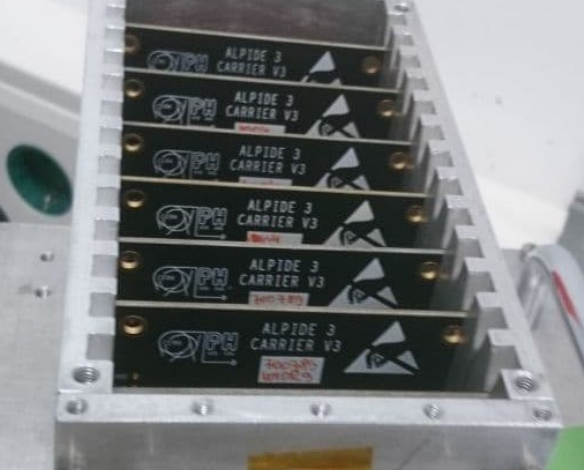
I report below results from the alignment of a 7 plane ALPIDE telescope where the sensors are inserted in place between metallic drilled inserts (so they are rather well fixed and the position/rotation should be quite well determined, given that it’s CNC machined). See the following picture:
I mention here that in the end for the efficiency analysis we used the association module, as not to bias the efficiency calculation (by requiring hits in every layer). We just used the alignment for all sensors at once since it should work very well, given no other material is in between.
For this setup, we had a colleague who has done 6 alignment steps (+ 1 pre alignment). By this, I mean get a new geometry file after each alignment which is then used as input for yet another corry run where tracks are re-fitted and a new alignment is found … and so on). Our sensors were operated at their nominal parameters (highly efficient, no noise). They were all 50um thin, no extra material in the telescope.
In a first step, the prealignment was done, using a Gaussian fit to find the mean and shift it to 0. The module AlignmentMillepede was then used with the following parameters:
[AlignmentMillepede]
exclude_dut = false
iterations = 2
dofs = true, true, false, true, true, true
residual_cut = .05mm
residual_cut_init = 1mm
number_of_stddev = 0
sigmas = 50um, 50um, 50um, .005rad, .005rad, .005rad
convergence = 1e-4
The prealignment does indeed find values ranging up to ~1 mm, and this understood by the placement of the sensors on the PCB and their insertion in the DAQ boards (below in the picture).
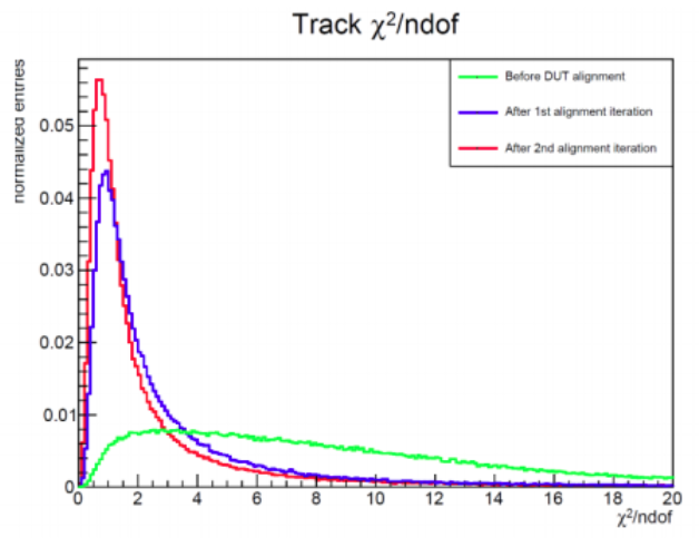
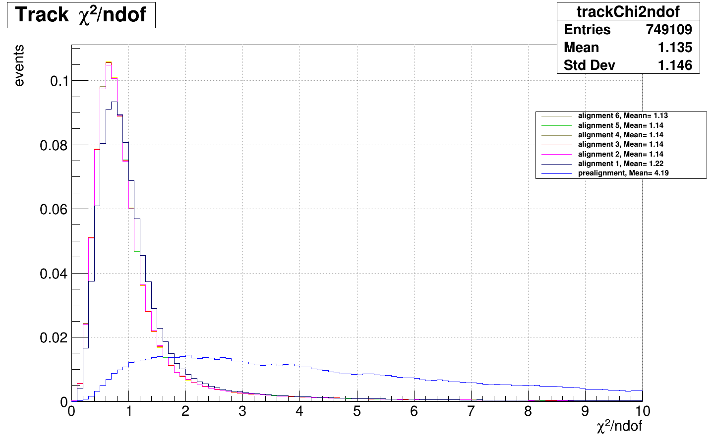
In the following picture I report the figure of merit, the track chi2/ndof for the runs:
One can see that after prealignment, a rather flat distribution is found, but still quite a few tracks have a chi2ndof <10. After a first alignment step, the track chi2ndof is already very good, with a mean of 1.22 A second step with track refitting improves this by a tiny bit (1.22 → 1.14) and is visible in the plot. Next iterations do not bring any improvement and are indistinguishable. (I mention at this point that by iterations I mean the number of alignment procedures, not the iteration parameter that the AlignmentMillepede module has, that was always kept at the value from above =2).
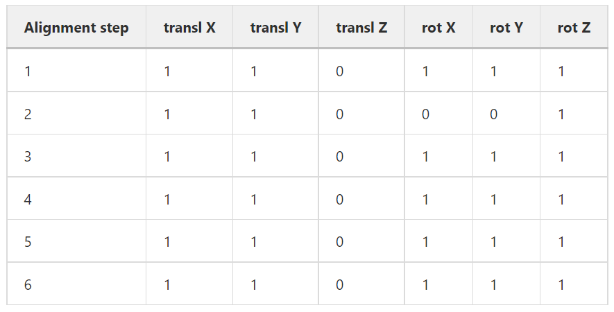
Below I report the values from the geometry files before/after such an iteration. There should be a total of 6 plots, for each of the degrees of freedom (translation X, Y, Z and rotation X, Y, Z). As can be seen from the AlignmentMillepede parameters, the z translation is not aligned, because this we serve as input in the initial geometry file and it should be well fixed. Therefore, this plot is not shown.
Also, since the tracking algorithm with translation X,Y and rotation X,Y,Z was stuck in a false minimum in the beginning, the second iteration step has the rotations in X and Y removed, while the Z is kept. As you will see later, the rot X and Y are minimal (< milli degree) (since the sensors are fixed in the metallic slots) and only the rotation around the Z axis has a higher impact.
This can be seen in the following table showing at which step what dofs were considered.
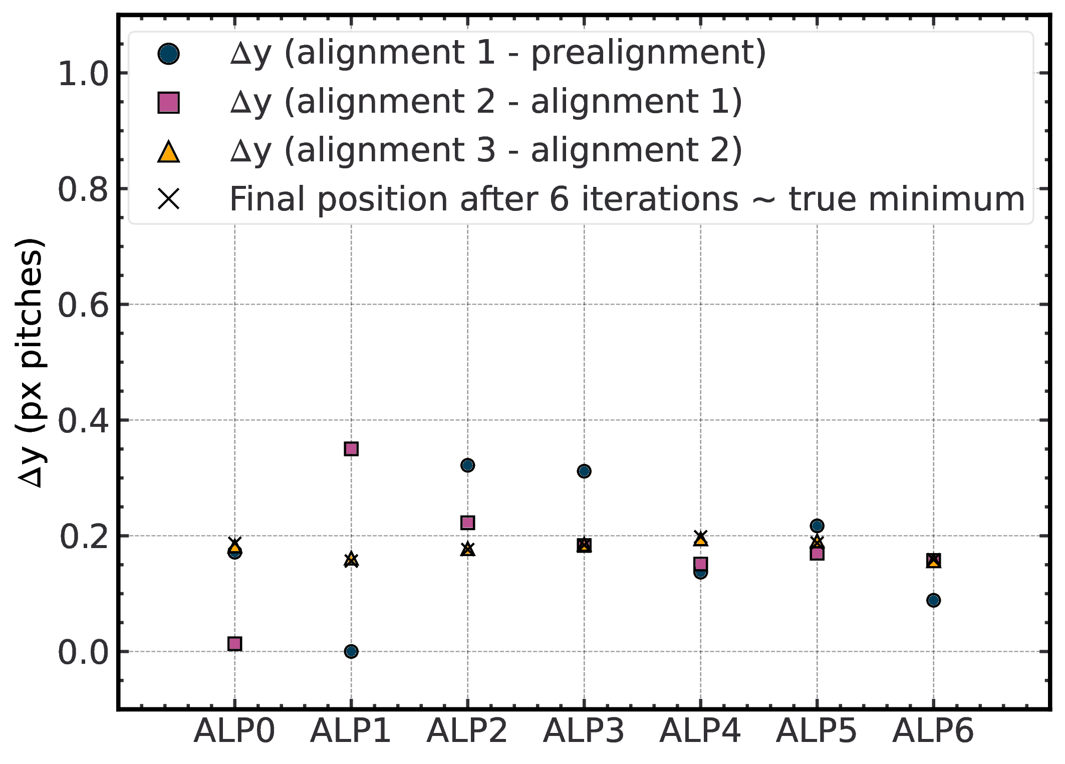
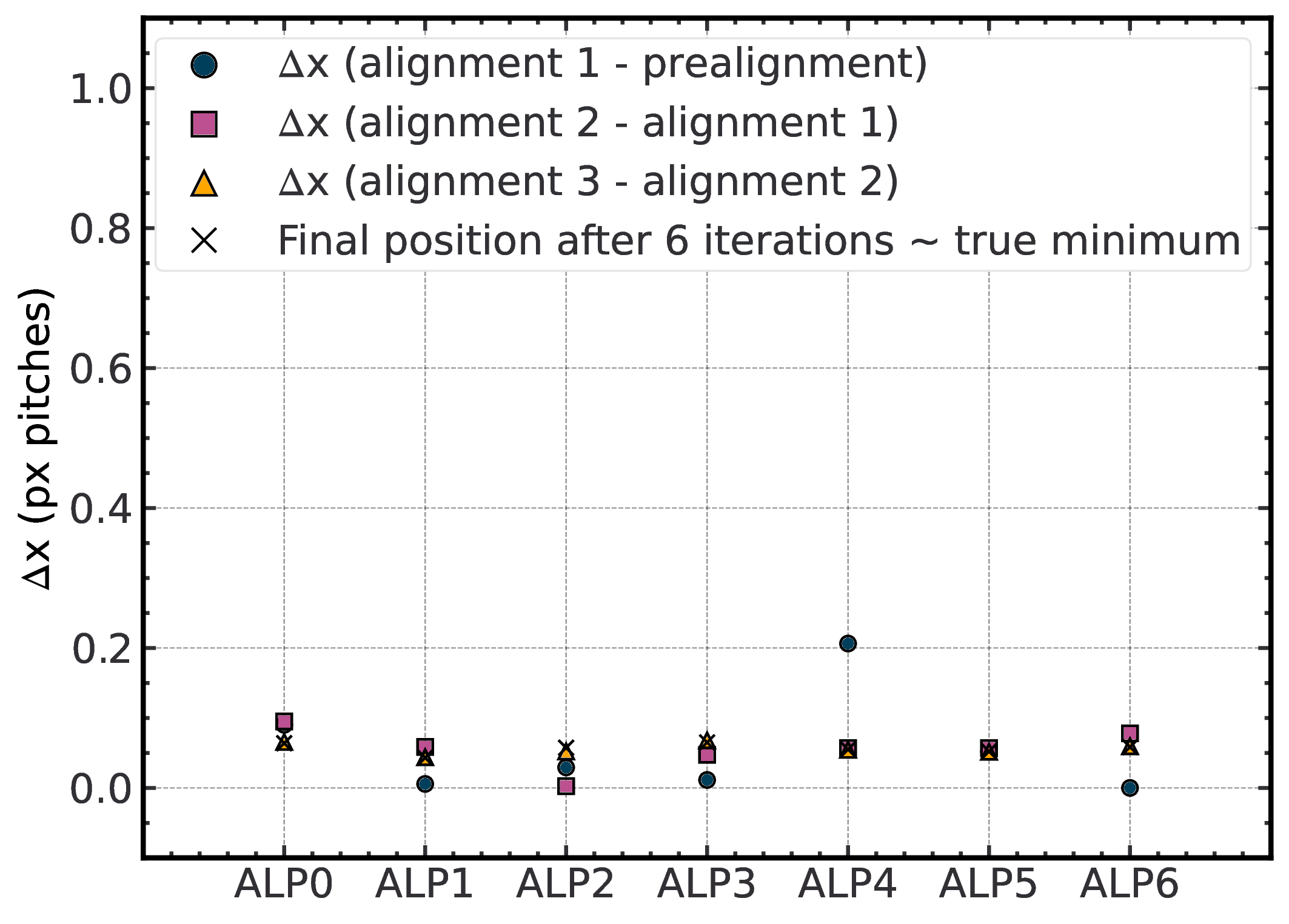
Next, I will plot for each of these degrees of freedom the difference between an alignment step and the next. I chose this instead of plotting the values directly, as some sensors had initial misalignment of eg: 1mm, while others had ~30um. Plotting those on the same scale would result in problems seeing the difference between iterations.
Here are the translations in X and Y. On the x axis are the 7 sensors, on the y axis I plotted this difference between alignments (check the legend to see what difference; I only plotted the first 3 alignments, since as I explained above the differences afterwards are minimal). This difference between alignments is expressed in pixel pitches (in the case of the ALPIDE 29.24 um in x and 26.88 in y).
What one can see is that the prealignment already does a good job in terms of translation. The changes between the first alignment and the prealignment is smaller than 20% of a pixel pitch (~6um) for x and smaller than 40% (~12um) for y. A second alignment will also add a correction, but afterwards diminishing returns. The positional difference after 6 iterations, I considered as sort of a true minimum is plotted as a cross and you can see that a third alignment does not improve anymore with respect to this position.
I did not plot the other alignments (4-6), but I observed something. Given the telescope resolution ~5um (and the inherent tracking error ~2-3um at the position of each sensor with GBL), the alignment algorithm will try to align again and again, always finding another minimum (close to the true one), but the changes are of the order of the resolution, as one would expect. So, one should be careful not to align too many times.
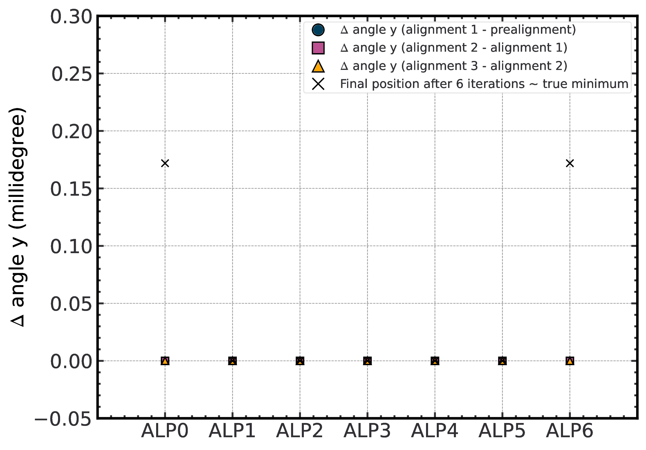
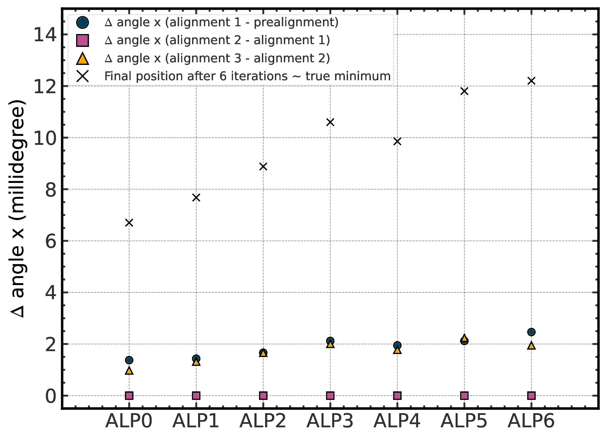
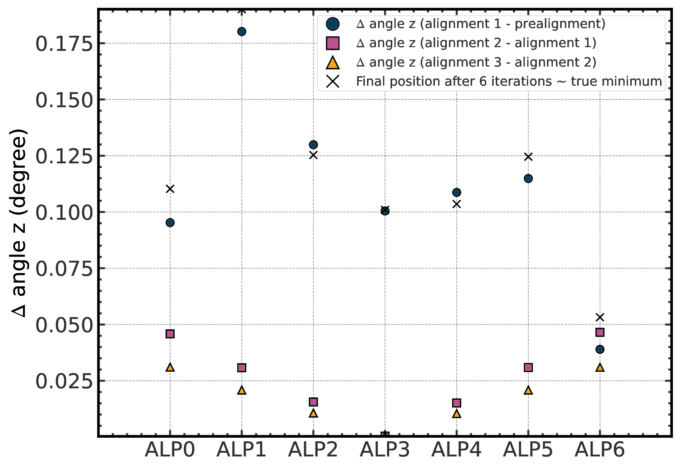
Now, for the rotations, here is the situation:
I will start by drawing your attention that for rotations around the x and y axes the units are in milli degrees, while for the rotations around the z axis this is expressed in degrees. So, the rotations around the z axis have a much higher impact.
The rotations around y are a bit special and currently not understood. Here, all values are 0 (the two crosses are due to rounding errors basically). In the config files, this dof is specified to be used, but the algorithm does not do it. We don’t understand why this is the case. For other testbeams, this works well.
For rotations around x, one can see the same behaviour as for translations, namely some improvement is possible (<2 milli degrees). If one then does more and more alignments on top of this already good one, the algorithm starts to have increased values (overfitting? migrating local minimum?)
A similar thing happens for rot z. Here, you see a large improvement from the prealignment (since in the prealignment only the translations are accounted for by the shift of the peak; nothing is done for the rotational dofs, so the first alignment is the first time these are accounted for). After this initial large improvement, the next two iterations are smaller, but again towards smaller values (showing that indeed one improves the alignment). After this second alignment, as explained above, the values start increasing.